Next: Datova struktura programu
Up: Weak formulation and boundary
Previous: Triangulation
Contents
In this section, the treatment of several types of boundary conditions is
explained in details. First, the boundary
 of the
computational domain
of the
computational domain  is decomposed into several disjoint parts. On
each part a different boundary condition is prescribed. Following the notation
from
FEMFLUID implementation, the following boundary parts are considered:
is decomposed into several disjoint parts. On
each part a different boundary condition is prescribed. Following the notation
from
FEMFLUID implementation, the following boundary parts are considered:
-
 - fixed wall,
-
 - inlet/Dirichlet part of boundary,
-
 - moving part of boundary with velocity
 ,
,![$ \\ [3mm]$](img17.png)
In this section a simplified analysis is carried only for
Navier-Stokes system of equations. This boundary condition is employed
only on moving meshes which follows the motion of the boundary
 . The numerical simulation on moving meshes can be treated
with the aid of ALE formulation. . The numerical simulation on moving meshes can be treated
with the aid of ALE formulation.
|
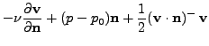
 - outlet,
|
do-nothing boundary condition (see, e.g., [4]),
|
-
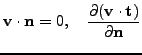
 - symmetry condition,
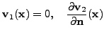
 - symmetry condition for boundary with the fixed
 -coordinate
  , i.e. the normal vector is
 ,
,
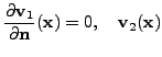
 - symmetry condition for boundary with the fixed
 coordinate
  , i.e. the normal vector is
 .
.
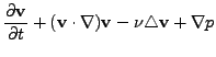
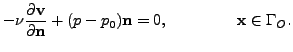
In order to describe the weak formulation we start from incompressible system
of Navier-Stokes equations. Here, the system of Navier-Stokes equations in the
form
is considered. In agreement the following boundary conditions are prescribed
on mutually disjoint parts of
 .
Here, we list the prescribed boundary conditions
.
Here, we list the prescribed boundary conditions
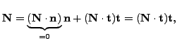
where
 is the unit outward normal to the boundary of
and
is the unit outward normal to the boundary of
and
 is the unit tangent vector on the boundary of
(oriented
in such a way, that the domain is on the left-hand side).
is the unit tangent vector on the boundary of
(oriented
in such a way, that the domain is on the left-hand side).
Condition (2) can be replaced by the well known do-nothing
condition
 |
(3) |
If the boundary
 is really the outlet part of the boundary
(t.j.
is really the outlet part of the boundary
(t.j.
 ), both conditions are equal. If this is not the case,
the boundary condition (2) rejects the kinetic energy coming from
the outlet part of boundary.
), both conditions are equal. If this is not the case,
the boundary condition (2) rejects the kinetic energy coming from
the outlet part of boundary.
Further, the space of test functions needs to be chosen in agreement with the
prescribed boundary conditions. The following conditions are considered :
The space  is defined by
Now, take a test function
 , multiply system
(1) and integrate over . For simplicity we
denote
, multiply system
(1) and integrate over . For simplicity we
denote
With the fact that
 on
on
 and by applying Green's theorem we get
step by step
and by applying Green's theorem we get
step by step
 |
(5) |
and similary
 |
(6) |
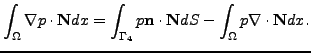
Further, for the convective term (
 from cotinuity equation)
where the tri-linear skew-symmetric form  reads
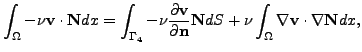
Finally, with the use of Eqs. 5,
6, 7 we get the weak
formulation of Navier-Stokes equations
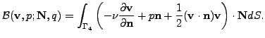
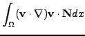
where on the left hand side there is - except the standard terms - also the
boundary integral
This form needs to rewritten with respect to the boundary conditions.
Consider now the different parts of the boundary
reads
Finally, with the use of Eqs. 5,
6, 7 we get the weak
formulation of Navier-Stokes equations
where on the left hand side there is - except the standard terms - also the
boundary integral
This form needs to rewritten with respect to the boundary conditions.
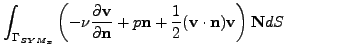
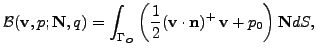
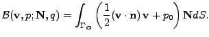
Consider now the different parts of the boundary  : first on
then on
: first on
then on
and similary on
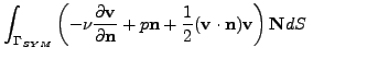
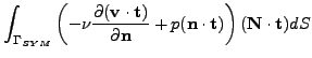
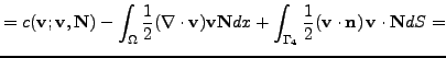
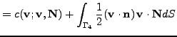
Finally, on
we write
so that
The following terms are included in term 
which differs from the case of do-nothing boundary condition, where
Next: Datova struktura programu
Up: Weak formulation and boundary
Previous: Triangulation
Contents
Petr Svacek
2007-06-02
![\includegraphics[width=0.7\textwidth]{bc_u0.eps}](img10.png)
![\includegraphics[width=0.2\textwidth]{bc_u1.eps}](img13.png)
![\includegraphics[width=0.8\textwidth]{bcWt.eps}](img18.png)
![\includegraphics[width=0.8\textwidth]{bc_out.eps}](img22.png)
![\includegraphics[width=0.4\textwidth]{bc_sym.eps}](img24.png)
![\includegraphics[width=0.35\textwidth]{bc_sym_y.eps}](img25.png)
![\includegraphics[width=0.22\textwidth]{bc_sym_x.eps}](img26.png)

![$\displaystyle { c (\mathbf{u}; \mathbf{v},\mathbf{w})}= {\int_\Omega \left[ \fr...
...f{w}- \frac12
(\mathbf{u}\cdot \nabla) \mathbf{w}\cdot \mathbf{v}\right] dx }.
$](img80.png)